Binding for ggplot2::geom_sf(), therefore it supports
only sf objects.
Arguments
- mapping
Set of aesthetic mappings created by
ggplot2::aes(). Seeggplot2::geom_sf()for details.- data
The data to be displayed in this layer. See
ggplot2::geom_sf()for details.- stat
The statistical transformation to use on the data for this layer. See
ggplot2::geom_sf()for details.- position
A position adjustment to use on the data for this layer. See
ggplot2::geom_sf()for details.- na.rm
If
FALSE, the default, missing values are removed with a warning. IfTRUE, missing values are silently removed.- show.legend
logical. Should this layer be included in the legends? See
ggplot2::geom_sf()for details.- inherit.aes
If
FALSE, overrides the default aesthetics, rather than combining with them. Seeggplot2::geom_sf()for details.- keep
numeric, proportion of points to retain (0.05-5.0; default 0.5). See Details.
- method
character, either
"voronoi"(default) or"straight", or just the first letter"v"or"s". See Details.- simplify
logical, if
TRUE(default) then the centerline will be smoothed withsmoothr::smooth_ksmooth()- ...
Other arguments passed on to
ggplot2::layer(). Seeggplot2::geom_sf()for details.
CRS
coord_sf() ensures that all layers use a common CRS. You can
either specify it using the crs param, or coord_sf() will
take it from the first layer that defines a CRS.
Combining sf layers and regular geoms
Most regular geoms, such as geom_point(), geom_path(),
geom_text(), geom_polygon() etc. will work fine with coord_sf(). However
when using these geoms, two problems arise. First, what CRS should be used
for the x and y coordinates used by these non-sf geoms? The CRS applied to
non-sf geoms is set by the default_crs parameter, and it defaults to
NULL, which means positions for non-sf geoms are interpreted as projected
coordinates in the coordinate system set by the crs parameter. This setting
allows you complete control over where exactly items are placed on the plot
canvas, but it may require some understanding of how projections work and how
to generate data in projected coordinates. As an alternative, you can set
default_crs = sf::st_crs(4326), the World Geodetic System 1984 (WGS84).
This means that x and y positions are interpreted as longitude and latitude,
respectively. You can also specify any other valid CRS as the default CRS for
non-sf geoms.
The second problem that arises for non-sf geoms is how straight lines
should be interpreted in projected space when default_crs is not set to NULL.
The approach coord_sf() takes is to break straight lines into small pieces
(i.e., segmentize them) and then transform the pieces into projected coordinates.
For the default setting where x and y are interpreted as longitude and latitude,
this approach means that horizontal lines follow the parallels and vertical lines
follow the meridians. If you need a different approach to handling straight lines,
then you should manually segmentize and project coordinates and generate the plot
in projected coordinates.
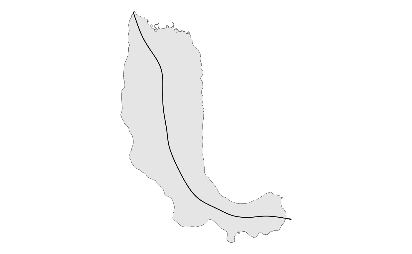
Examples
# \donttest{
library(sf)
library(ggplot2)

lake <-
  sf::st_read(
    system.file("extdata/example.gpkg", package = "centerline"),
    layer = "lake",
    quiet = TRUE
  )

ggplot() +
  geom_sf(data = lake) +
  geom_cnt(
    data = lake,
    keep = 1,
    simplify = TRUE
  ) +
  theme_void()

# }
# }