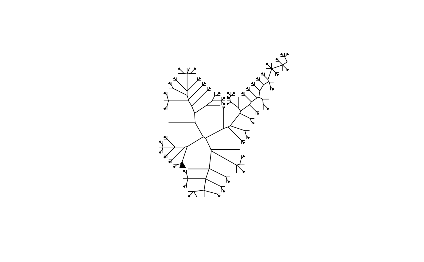
This function generates skeletons of closed polygon objects. Optional
boundary anchors can be attached as exact terminal graph nodes so that
cnt_path() can start or end at those points without nearest-node snapping.
Arguments
- input
sf,sfc,SpatVector, orgeos_geometrypolygons object- keep
numeric, proportion of points to retain (0.05-5.0; default 0.5). See Details.
- method
character, either
"voronoi"(default) or"straight", or just the first letter"v"or"s". See Details.- anchors
NULL(default) or boundaryPOINTgeometries of the same spatial class and CRS asinput. When supplied, each point must lie on exactly one polygon-part boundary (exterior or hole ring). Withmethod = "voronoi"andkeep < 1, accepted anchors are injected as exact exterior/hole ring vertices before protected simplification so they participate ingeos_unique_points()as Voronoi sites (the achieved vertex count may exceed the nominalkeepdensity). Connector validation and clipping then use that prepared polygon. Withkeep >= 1, anchors are not injected and the ordinary no-op or densify site set is retained. In all cases anchors are also attached by a direct interior connector so they remain explicit degree-one graph terminals. Attribute columns onanchorsare ignored; the returned skeleton still inherits polygon attributes exactly as without anchors.
Details
Polygon simplification/densification
If
keep = 1, no transformation will occur. The function will use the original geometry to find the skeleton.If the
keepparameter is below 1, then thegeos::geos_simplify()function will be used. So the original input geometry would be simplified, and the resulting skeleton will be cleaner but maybe more edgy. The current realisation of simplification is similar (but not identical) tormapshaper::ms_simplify()one with Douglas-Peuker algorithm. However, due togeossuperpower, it performs several times faster. If you find that the built-in simplification algorithm performs poorly, tryrmapshaper::ms_simplify()first and then find the polygon skeleton withkeep = 1, i.e.cnt_skeleton(rmapshaper::ms_simplify(polygon_sf), keep = 1)If the
keepis above 1, then the densification algorithm is applied using thegeos::geos_densify()function. This may produce a very large object if keep is set more than 2. However, the resulting skeleton would potentially be more accurate.
Skeleton method
If
method = "voronoi"(default), the skeleton will be generated using thegeos::geos_voronoi_edges()function. This is application of the Voronoi diagram algorithm (Voronoi, 1908). A Voronoi diagram partitions space into regions based on the distance to the polygon's vertices. The edges of these cells form a network of lines (skeletons) that represent the structure of the polygon while preserving its overall shape.If
method = "straight", the skeleton will be generated using theraybevel::skeletonize()function. See https://www.tylermw.com/posts/rayverse/raybevel-introduction.html
Boundary anchors
When anchors is supplied, each accepted boundary point is matched to
the original unnested polygon-part boundary first. For
method = "voronoi" and keep < 1, those anchors are then
injected as exact ring vertices and the polygon is simplified with those
vertices protected, so Voronoi generation, clipping, coverage tests, and
connector construction all share one prepared domain. With
keep >= 1, or with method = "straight", the ordinary skeleton
is still built from the (uninjected) polygon under the existing
keep/method behavior and anchors attach only by connector.
Candidate junctions are scored among the nearest skeleton junctions (by
planar Euclidean distance and turn angle; use projected coordinates when
that ranking must be spatially meaningful). A full chord to a pre-existing
degree-at-least-three junction is preferred; if every such chord crosses
other skeleton branches, the connector is clipped to the first skeleton hit
along the same ray (mid-edge T-junction). Calls fail when an anchor is
off-boundary, shared by multiple parts, duplicated, or has no valid
connector.
References
Voronoi, G. (1908). Nouvelles applications des paramètres continus à la théorie des formes quadratiques. Journal für die reine und angewandte Mathematik, 134, 198-287. doi:10.1515/crll.1908.134.198
Examples
library(sf)
polygon <-
sf::st_read(system.file("extdata/example.gpkg", package = "centerline"),
layer = "polygon",
quiet = TRUE
)
plot(polygon)
 pol_skeleton <- cnt_skeleton(polygon)
plot(pol_skeleton)
pol_skeleton <- cnt_skeleton(polygon)
plot(pol_skeleton)
 # Attach exact boundary terminals for routing
points <- sf::st_read(
system.file("extdata/example.gpkg", package = "centerline"),
layer = "polygon_points",
quiet = TRUE
)
boundary <- sf::st_boundary(polygon)
anchors <- points[
as.numeric(sf::st_distance(points, boundary)) == 0,
]
anchored <- cnt_skeleton(polygon, keep = 1, anchors = anchors)
plot(anchored)
# Attach exact boundary terminals for routing
points <- sf::st_read(
system.file("extdata/example.gpkg", package = "centerline"),
layer = "polygon_points",
quiet = TRUE
)
boundary <- sf::st_boundary(polygon)
anchors <- points[
as.numeric(sf::st_distance(points, boundary)) == 0,
]
anchored <- cnt_skeleton(polygon, keep = 1, anchors = anchors)
plot(anchored)